MCMC with matryoshka and zeus

In this example we demonstrate how to exploit the batch preidctions of matryoshka when running an MCMC with zeus.

We start by import all the packages required for this example.

import numpy as np
import matryoshka.emulator as Matry
import matryoshka.halo_model_funcs as MatryHM
from matryoshka.training_funcs import dataset
import matplotlib.pyplot as plt
from scipy.interpolate import interp1d
from scipy.stats import multivariate_normal
from scipy.optimize import minimize
import zeus
import time

Next we initalise the \(T(k)\) component emulator. This is very simple and can be done with the .Transfer() emulator class. Upon initalisation all weights for the neural networks (NNs) are loaded meaning that no re-training is required before making predictions.

# For environments with tensorflow>=2.5 this cell triggers a set of
# of warnings as the provided weights were produced with tensorflow==2.4.0
# Predictions can still be made using these weight, however new weights
# files will be provided in future versions that wont trigger these warnings.
TransferEmu = Matry.Transfer()

2023-10-31 16:46:46.006074: I tensorflow/core/platform/cpu_feature_guard.cc:142] This TensorFlow binary is optimized with oneAPI Deep Neural Network Library (oneDNN) to use the following CPU instructions in performance-critical operations:  AVX2 FMA
To enable them in other operations, rebuild TensorFlow with the appropriate compiler flags.

We next select a cosmology at random from the matryoshka test set. This randomly selected cosmology will be our “truth”.

# We load X_sigma instead of X_transfer here simply because it conatins all 7 cosmological parameters.
# X_transfer excludes sigma8 and ns.
valX = dataset("sigma", "val", "X")
valY = dataset("transfer", "val", "Y")

# Set seed so example is reproducable.
np.random.seed(42)
truth_id = np.random.choice(valX.shape[0])
truth_id

1126

COSMO_true = valX[truth_id]
Tk_true = valY[truth_id]
print("True cosmology:")
#Make string with true cosmology
cosmo_string = "Om:{a}, Ob:{b}, sigma8:{c}, h:{d}, ns:{e}, Neff:{f}, w0:{g}".format(
    a=COSMO_true[0], # Om
    b=COSMO_true[1], # Ob
    c=COSMO_true[2], # Sigma8
    d=COSMO_true[3], # h
    e=COSMO_true[4], # ns
    f=COSMO_true[5], # Neff
    g=COSMO_true[6] # w0
)
print(cosmo_string)

True cosmology:
Om:0.33096736776710545, Ob:0.052357134319917294, sigma8:0.7740745054892728, h:0.6452520706158401, ns:0.9634715635096555, Neff:4.006127861404566, w0:-0.8598609356831605

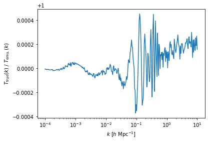
As a quick test we can see how the prediction from the \(T(k)\) component emulator compares to the truth when the true cosmological parameters are used as input.

Tk_pred = TransferEmu.emu_predict(
    COSMO_true,
    mean_or_full="mean"
)

plt.semilogx(
    TransferEmu.kbins,
    Tk_true/Tk_pred[0],
    label = "Truth"
)

plt.xlabel(r"$k \ [h \ \mathrm{Mpc}^{-1}]$")
plt.ylabel(r"$T_\mathrm{true}(k) \ / \ T_\mathrm{emu.}(k)$")

plt.show()

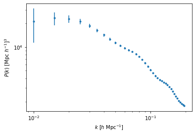
To generate a mock signal we can use in our MCMC, we calculate the linear matter power spectrum \(P_L(k) = A_s k^{n_s}T^2(k)\). This is clearly an unrealistic example, the linear matter power spectrum is not something we will observe, it serves as a simple example that will convergence quickly whilst using all the cosmological parameters of our model.

# Impose a range that would be more realistic if we were considering galaxy clustering.
k_obs = np.arange(
    0.01,
    0.2,
    0.005
)

# Calculate matter PS from transfer function, sigma8, and ns
power_true = interp1d(
    TransferEmu.kbins,
    MatryHM.power0_v2(
        TransferEmu.kbins,
        Tk_true,
        sigma8=COSMO_true[2],
        ns=COSMO_true[4]
    )[0]
)(k_obs)

# Define a very simple scale dependent measurement noise.
noise = k_obs**(-2)

# Make plot
plt.errorbar(
    k_obs,
    power_true,
    yerr=noise,
    linestyle='none',
    marker='.'
)

# Make loglog
plt.xscale('log')
plt.yscale('log')

plt.xlabel(r"$k \ [h \ \mathrm{Mpc}^{-1}]$")
plt.ylabel(r"$P(k) \ [\mathrm{Mpc} \ h^{-1}]^3$")

plt.show()

Now we can think about defining our prior and likelihood to be used in the MCMC.

For the prior we use a multivariate Gaussian prior that is defined by the matryoshka training samples. This prior associates low probability to regions of the parameter space that are not covered by training data.

trainX = dataset("sigma", "train", "X")

mvn = multivariate_normal(
    trainX.mean(axis=0),
    np.cov(trainX, rowvar=False)
)

def log_prior(theta):
    '''
    Evaluation of the log prior.

    Args:
        theta (array) : Model parameters for which the prior should be evaluated.
         Should have shape ``(n_samples, n_params)``.
    '''

    return mvn.logpdf(theta[:,:])

Next we define a Gaussian likelihood with the form

\[\ln{\mathcal{L}(d|\theta)}=-\frac{1}{2}\frac{(P-P'(\theta))^2}{\sigma^2}.\]

Where \(P\) is our power_true, \(P'(\theta)\) is the emulator prediction for the parameters \(\theta\), and \(\sigma\) is our noise. We construct this function such that it expects multiple parameter sets to evaluate, exploiting the batch prediction speed from matryoshka.

def log_like(theta, obs_pow, noise):
    '''
    Evaluation of log likelihood.

    Args:
        theta (array) : Model parameters for which the prior should be evaluated.
         Should have shape ``(n_samples, n_params)``.
        obs_pow (array) : The power spectrum that is being used for inference.
        noise (array) : The uncertainty associated to ``obs_pow``.
    '''

    # Predict transfer functions for each sample in theta
    preds_T = TransferEmu.emu_predict(
        theta[:,[0,1,3,5,6]],
        mean_or_full='mean'
    )

    # Calculate matter power for each sample in theta
    preds_power = interp1d(
        TransferEmu.kbins,
        MatryHM.power0_v2(
            TransferEmu.kbins,
            preds_T,
            sigma8=theta[:,2],
            ns=theta[:,4]
        )
    )(k_obs)

    # Calculate residual
    res = obs_pow - preds_power

    return -0.5*np.sum(res**2/noise**2, axis=1)

The final function we need before runnig our MCMC combines the log-likelihood and the log-prior to calculate the log-probability.

def log_prob(theta, obs_pow, noise):
    '''
    Evaluation of unnormalised log posterior.

    Args:
        theta (array) : Model parameters for which the prior should be evaluated.
         Should have shape ``(n_samples, n_params)``.
        obs_pow (array) : The power spectrum that is being used for inference.
        noise (array) : The uncertainty associated to ``obs_pow``.
    '''

    # Make sure theta is an array
    theta = np.array(theta)

    # Evaluate log prior
    lp = log_prior(theta)

    # Evaluate the log likelihood
    ll = log_like(theta, obs_pow, noise)

    return ll+lp

# We also define a function for the negative log_prob, this will be used with the minimize function from scipy so
# does not exploit batch predictions.
def neg_log_prob(theta, obs_pow, noise):
    '''
    Evaluation of the negative unnormalised log posterior.

    Args:
        theta (array) : Model parameters for which the prior should be evaluated.
         Should have shape ``(n_samples, n_params)``.
        obs_pow (array) : The power spectrum that is being used for inference.
        noise (array) : The uncertainty associated to ``obs_pow``.
    '''

    # Make theta 2d
    theta = np.atleast_2d(theta)

    return -(log_prob(theta, obs_pow, noise))

As the title of this notebook suggests, we will be using zeus to do our MCMC. zeus is an ensemble sampler, as such requires us to generate inital positions for an ensemble of walkers. For this example we generate the walker positions as small perturbations from the MAP position.

# Minimise the neg log prob
results = minimize(
    neg_log_prob, # function
    trainX.mean(axis=0), # inital guess
    args=(
        power_true,
        noise
    ),
    options={
        'disp': True, # Print summary of results
        "maxiter": 100000 # Impose a max number of iterations before termination.
    },
    method='Nelder-Mead'
)

print("===================")
print("Maximum likelihood cosmology:")
ml_string = "Om:{a}, Ob:{b}, sigma8:{c}, h:{d}, ns:{e}, Neff:{f}, w0:{g}".format(
    a=results.x[0],
    b=results.x[1],
    c=results.x[2],
    d=results.x[3],
    e=results.x[4],
    f=results.x[5],
    g=results.x[6]
)
print(ml_string)
print("===================")
print("True cosmology:")
print(cosmo_string)

# Specify a number of walkers
nwalk = 20

#Define the number of dimensions
ndim = 7


init_pos = results.x+1e-3*np.random.randn(nwalk, ndim)

Optimization terminated successfully.
         Current function value: -18.293803
         Iterations: 392
         Function evaluations: 632
===================
Maximum likelihood cosmology:
Om:0.33214647391403196, Ob:0.05287365754374555, sigma8:0.7739539864442344, h:0.6488262308757469, ns:0.9570062742299779, Neff:3.8717047190077336, w0:-0.9054214466605468
===================
True cosmology:
Om:0.33096736776710545, Ob:0.052357134319917294, sigma8:0.7740745054892728, h:0.6452520706158401, ns:0.9634715635096555, Neff:4.006127861404566, w0:-0.8598609356831605

We can now run our MCMC, we run for 1000 steps, this should be more that \(10\times\) the autocorrelation time for most examples.

# Define the sampler
sampler = zeus.EnsembleSampler(
    nwalk,
    ndim,
    log_prob,
    args=(
        power_true,
        noise
    ),
    vectorize=True # matryoshka is more efficent when using vectorisation
)

# Start time
start = time.time()

# Start sampler
sampler.run_mcmc(init_pos, 1000, progress=True)

# End time
end = time.time()

# Print total number of evaluations in run time
print("{a} likelihood evaluations in {b} minutes.".format(a=sampler.ncall, b=np.round((end-start)/60,1)))

Initialising ensemble of 20 walkers...
Sampling progress : 100%|██████████████████████████████████████████████████████| 1000/1000 [02:53<00:00,  5.76it/s]

97652 likelihood evaluations in 2.9 minutes.

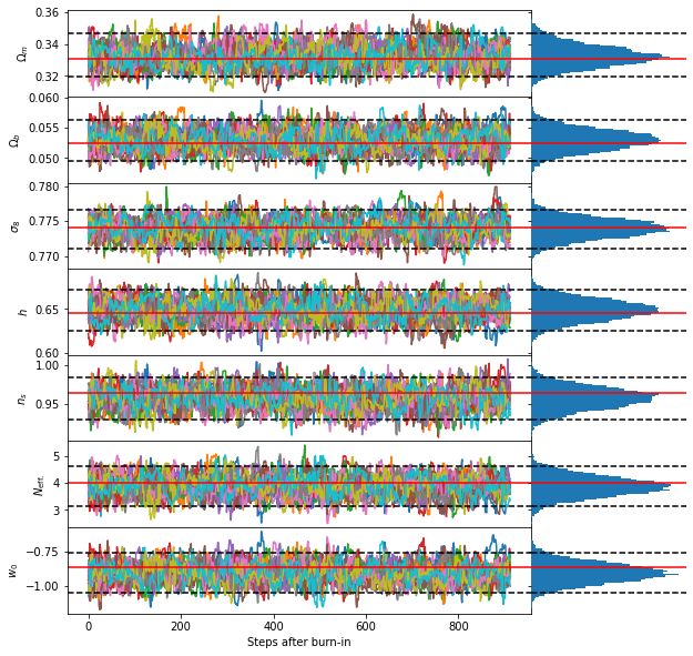
Once the MCMC has finished we can examine our chains and resulting posterior distributions.

# For this example we say that the chain is burnt-in once we have reached more than 5X the autocorrelation time.
# We only keep the samples after we have burnt-in.
chain = sampler.get_chain(
    flat=False,
    discard=int(sampler.act.max()*5)
)

# Define plot
fig, ax = plt.subplots(
    7,
    2,
    figsize=(10,10),
    gridspec_kw={
        'width_ratios':[3,1]
    },
    sharex='col',
    sharey='row')

# Define parameter labels
labels = [
    r"$\Omega_m$",
    r"$\Omega_b$",
    r"$\sigma_8$",
    r"$h$",
    r"$n_s$",
    r"$N_\mathrm{eff.}$",
    r"$w_0$"]

# Loop over the number of parameters
for i in range(7):
    # Plot parameter chain
    ax[i,0].plot(chain[:,:,i])

    # Set label
    ax[i,0].set_ylabel(labels[i])

    # Plot posterior
    ax[i,1].hist(
        chain[:,:,i].flatten(), # Combine chains from all walkers
        bins=50,
        orientation='horizontal'
    )

    # Remove frame and ticks for posterior
    ax[i,1].set_frame_on(False)
    ax[i,1].set_xticks([])

    # Loop over chain and posterior plot
    for j in range(2):
        # Plot truth
        ax[i,j].axhline(COSMO_true[i], color='red')
        for q in [0.025, 0.975]:
            # Plot 95% CI
            ax[i,j].axhline(np.quantile(chain[:,:,i].flatten(), q), color='k', linestyle='--')

ax[-1,0].set_xlabel("Steps after burn-in")
plt.subplots_adjust(hspace=0., wspace=0.)
plt.show()